When we run a SQL statement in Management Studio, if SQL Server thinks the statement would benefit from an index it will give us that recommendation right in Management Studio. SQL Server doesn’t just make these recommendations in Management Studio, but anytime a SQL statement is run, and these recommendations are logged to a series of DMVs known as the missing_index DMVs. We don’t want to automatically create every index that is recommended in this series of views, but looking at these results can help us find an index that we may have otherwise overlooked. The below query will join these views together and give us some statistics about the recommendations.
SELECT TableName=OBJECT_NAME(d.object_id),
    d.equality_columns,
    d.inequality_columns,
    d.included_columns,
    s.user_scans,
    s.user_seeks,
    s.avg_total_user_cost,
    s.avg_user_impact,
    AverageCostSavings = ROUND(s.avg_total_user_cost * (s.avg_user_impact/100.0), 3),
    TotalCostSavings = ROUND(s.avg_total_user_cost * (s.avg_user_impact/100.0) * (s.user_seeks + s.user_scans),3)
FROM sys.dm_db_missing_index_groups g
INNER JOIN sys.dm_db_missing_index_group_stats s
    ON s.group_handle = g.index_group_handle
INNER JOIN sys.dm_db_missing_index_details d
    ON d.index_handle = g.index_handle
WHERE d.database_id = db_id()
ORDER BY TotalCostSavings DESC, TableName
Now when you run this query and pull this list up, what you don’t want to do is just start working your way down the list and creating an index for each row in this result set. This is because SQL Server has a tendency to recommend an index to optimize every individual statement, and if you did that you would be in an over-index situation, which would slow down all of your DML statements against your tables. Instead, what you want to do is to scan through the results and for each table you’ll be able to pick out some patterns of index recommendations across similar columns, and then you can combine this information with your knowledge of how your application works to come up with the right set of indexes for each table.
A Sample Review
Below example shows that SQL Server could have performed an index seek operation against below first index 146978 times had the index existed.
Important Notes:
TableName: It is the table that the index recommendation is for.
Equality Columns-Inequality Columns-Included Columns: These columns containing information about what columns a potential index would be created across, and column names are given to us in a comma-separated list within each of these columns. Mainly, we’re going to be looking at the column called equality_columns, because most WHERE clauses and JOIN clauses are based on an equality relationship.
User Scans-User Seeks: We have some stats about why SQL Server thinks this index would be a good idea. These two columns here, user_scans and user_seeks, represent the number of times that SQL Server could have used this index had this index existed.
Avg Total User Cost: It is average cost of the statement without the index existing.
Avg User Impact: It tells us the percentage that SQL Server thinks that this cost would have been reduced if we would have had this index.
Average Cost Savings: It gives us the average cost savings per statement we would have by having this index.
Total Cost Savings: It gives us the total savings we would have across all statements that could benefit from having the index, so this value is useful to sort these results to get an idea of what the most impactful index to create might be.
SQL Server has to maintain any indexes you create on your tables, by updating an index every time a DML statement is executed against the table. So while an index will greatly speed up a query, there is a slight performance penalty in terms of executing a DML statement against the table. Therefore, we want to make sure our application is using all of the indexes we have created in our database, because otherwise we are paying the cost of maintaining an index which is not giving us any benefit. And we can do this with a query that looks like below, which uses the dm_db_index_usage_stats DMV in conjunction with the sys_indexes system view.
SELECT
[DatabaseName]=DB_Name(db_id()),
o.name AS TableName,
i.name AS IndexName,
[IndexType] = i.type_desc,
[TotalUsage] = IsNull(user_seeks, 0) + IsNull(user_scans, 0) + IsNull(user_lookups, 0),
--i.index_id AS IndexID,
dm_ius.user_seeks AS UserSeek,
dm_ius.user_scans AS UserScans,
dm_ius.user_lookups AS UserLookups,
dm_ius.user_updates AS UserUpdates,
--p.TableRows,
'DROP INDEX ' + QUOTENAME(i.name)
+ ' ON ' + QUOTENAME(s.name) + '.'
+ QUOTENAME(OBJECT_NAME(dm_ius.OBJECT_ID)) AS 'drop statement'
FROM sys.dm_db_index_usage_stats dm_ius
INNER JOIN sys.indexes i ON i.index_id = dm_ius.index_id
AND dm_ius.OBJECT_ID = i.OBJECT_ID
INNER JOIN sys.objects o ON dm_ius.OBJECT_ID = o.OBJECT_ID
INNER JOIN sys.schemas s ON o.schema_id = s.schema_id
INNER JOIN (SELECT SUM(p.rows) TableRows, p.index_id, p.OBJECT_ID
FROM sys.partitions p GROUP BY p.index_id, p.OBJECT_ID) p
ON p.index_id = dm_ius.index_id AND dm_ius.OBJECT_ID = p.OBJECT_ID
WHERE OBJECTPROPERTY(dm_ius.OBJECT_ID,'IsUserTable') = 1
AND dm_ius.database_id = DB_ID()
AND i.type_desc = 'nonclustered'
AND i.is_primary_key=0
AND i.is_unique_constraint=0
ORDER BY (dm_ius.user_seeks + dm_ius.user_scans + dm_ius.user_lookups) ASC
A Sample Review
The indexes in the first two rows below have been updated in DML (UserUpdates) processes even though they have never been used (Seek=0).
These indexes can be dropped after application team approval.
Important Notes:
Each represent the number of times respectively that the index has been used for those types of operations since SQL Server was last restarted.
User Seeks: SQL Server is traversing the B-Tree structure of the index to perform a lookup on a key. This is the operation we want to see. SQL Server is using the index as intended.
User Scans: SQL Server is reading the entire index to find the value(s) it wants.
If this is a Clustered Index, that means SQL Server is reading the entire table.
If this is a Non-Clustered Index, all of the index keys have to be read. This is much more expensive than a seek operation
User Lookups: These are lookup operations against the table, typically when SQL Server is looking up a row in the clustered index structure of a table.
User Updates: It gives the maintenance cost of the index. That is how many time a DML statement has caused this index to need to be updated.
You definitely have tablespace occupancy alarms in the databases you have managed and you are monitoring them.
Despite that, I highly recommend you to follow the items below so that you do not get an ORA-XXXXX Unable to Extend error one day and experience service interruption.
1. Creating an alarm for the max next extent sizes of objects at the tablespace level approaching the largest free contiguous extent size on the same tablespace. I am attaching the alarm SQL that I have prepared to this document.
2. If there is none, the critical ORA-XXXXX errors, which are reflected in the alertlog, must be sent to the relevant persons via e-mail.
3. Pro-actively following the tablespace fragmentations and performing the necessary maintenance work
LARGEST FREE CONTIGUOUS EXTENT SIZE ALARM
ALARM SQL
SELECT SEG.TABLESPACE_NAME,
       SEG.MAX_OBJECT_NEXT_EXTENT_SIZE,
       DFS.LARGEST_FREE_CONTIGUOUS_EXTENT_SIZE,
       CASE
           WHEN SEG.MAX_OBJECT_NEXT_EXTENT_SIZE / 2 >
                LARGEST_FREE_CONTIGUOUS_EXTENT_SIZE
           THEN
               'FREE CONTIGUOUS EXTENT SIZE IS LESS THAN HALF OF THE MAX OBJECT NEXT SIZE'
           ELSE
               'THERE IS SUFFICIENT FREE CONTIGUOUS EXTENT SIZE'
       END
           MESSAGE
  FROM (  SELECT SEG.TABLESPACE_NAME,
                 MAX (SEG.NEXT_EXTENT)     MAX_OBJECT_NEXT_EXTENT_SIZE
            FROM DBA_SEGMENTS SEG
        GROUP BY SEG.TABLESPACE_NAME) SEG,
       (  SELECT DFS.TABLESPACE_NAME,
                 MAX (DFS.BYTES)     LARGEST_FREE_CONTIGUOUS_EXTENT_SIZE
            FROM DBA_FREE_SPACE DFS
        GROUP BY DFS.TABLESPACE_NAME) DFS
 WHERE SEG.TABLESPACE_NAME = DFS.TABLESPACE_NAME
SAMPLE OUTPUT OF SQL
TROUBLESHOOTING STEPS
An “unable to extend” error is raised when there is insufficient contiguous space available to extend a segment.
1- Information needed to resolve UNABLE TO EXTEND errors
In order to address UNABLE TO EXTEND errors the following information is needed:
a- Determine the largest contiguous space available for the tablespacewith the error
The below query returns the largest available contiguous chunk of space.
SELECT max(bytes) FROM dba_free_space WHERE tablespace_name = '<tablespace name>';
If this query is done immediately after the failure, it will show that the largest contiguous space in the tablespace is smaller than the next extent the object was trying to allocate.
b- Determine NEXT_EXTENT size
DBA_SEGMENTS – NEXT_EXTENT: Size in bytes of the next extent to be allocated to the segment
SELECT NEXT_EXTENT FROM DBA_SEGMENTS WHERE SEGMENT_NAME = <segment name> AND SEGMENT_TYPE = <segment type> AND OWNER = <owner> AND TABLESPACE_NAME = <tablespace name>;
2- Possible Solutions
There are several options for resolving UNABLE TO EXTEND errors.
a- Manually Coalesce Adjacent Free Extents
The extents must be adjacent to each other for this to work.
ALTER TABLESPACE <tablespace name> COALESCE;
b- Defragment the Tablespace
If you would like more information on fragmentation, the following documents are available from Oracle Support.
Script to Detect Tablespace Fragmentation – Note 1020182.6 Script to Report Tablespace Free and Fragmentation – Note 1019709.6 Overview of Database Fragmentation – Note 1012431.6 Recreating Database Objects – Note 30910.1
You might have 46MB free space on tablespace but the largest contiguous extent size might only be 100KB.
It is possible that you have lots of free extents that are next to each other – you can try running “alter tablespace T coalesce” to see if that increases the largest free contiguous extent size in that tablespace.
This error does not necessarily indicate whether or not you have enough space in the tablespace, it merely indicates that Oracle could not find a large enough area of free contiguous space in which to fit the next extent.
There is possibility that the datafile is hit by fragmentation . Please check it out and remove the fragmentation.
You might have LOTS of free space available in the tablespace, but the largest contiguous extent might be too small.
You will need to check what is the NEXT extent size for that index and what is the largest contiguous extent size.
Your tablespace might have fragmented. Even though you have space in the tablespace its not able to extend. Please use the below note ids.
Script to Detect Tablespace Fragmentation (Doc ID 1020182.6)
Script to Report Tablespace Free and Fragmentation (Doc ID 1019709.6)
USEFUL NOTES
Space Management
It is very important to maximizing usage of your database. Over time your database can become fragmented. This will affect the performance and resources of your database. Here are some symptoms that may indicate fragmentation in your database:
If you are receiving any ORA errors regarding allocation of extents or space
If you look in dba_free_space and you see that there is a lot of free space left in that tablespace but you are receiving space errors.
What is fragmentation?
When a tablespace is fragmented, there may be a lot of free space in the tablespace, but they are in such small pieces that Oracle cannot use them. When an object needs a next extent, Oracle has to allocate one contiguous extent. If you do not have one chunk of free space that is large enough for the extent, Oracle will return an error. Your tablespace may have smaller pieces of free space that may add up to the size of the next extent, but Oracle cannot divide the next extent of the object into smaller pieces to fit into the free space.
There are two types of fragmentation. The tablespace may have two pieces of free space but in between the two, there is a permanent object. There is no way to coalesce those two free extents. Another type of fragmentation occurs when the tablespace has two pieces of free space that are adjacent to each other, but they are separate. With this type of fragmentation, Oracle’s SMON will coalesce the two extents into one large extent of free space. This automatic coalescing is new in Oracle7 and on.
What is Oracle Extent?
An extent is a logical unit of database storage space allocation made up of a number of contiguous data blocks. One or more extents in turn make up a segment. When the existing space in a segment is completely used, Oracle allocates a new extent for the segment.
Logical and Physical Database Structures
Segments, Extents, and Data Blocks Within a Tablespace
If you need to historically check the resource usage (Example: DB CPU) according to the services in the Oracle database, you can use the following SQL that I have prepared by revising it according to your needs.
Please note that the query was confirmed by Connor on asktom.
/*
REFERENCES:
1. https://asktom.oracle.com/pls/apex/f?p=100:11:::::P11_QUESTION_ID:9532872700346037612

2. https://docs.oracle.com/en/database/oracle/oracle-database/19/refrn/V-SERVICE_STATS.html#GUID-15943516-7233-4F2C-A2BE-7D6A766CBDDA
VALUE
For statistics that measure time (such as the DB CPU), this column displays a cumulative value in microseconds.
For other statistics that do not measure time (such as execute count) this column displays the appropriate numeric value for the statistic.
*/

/*
Query Logic
1. VALUE: The statistical value of the days in the time period specified at the instance level is found by subtracting the minimum value from the maximum value. Since VALUE is cumulative.
2. Group by is done according to SERVICE_NAME and STAT_NAME. Thus, the values of the instances are collected at the SERVICE_NAME and STAT_NAME levels for the specified time period.
3. SUM_VALUE column is created by summing up the relevant statistical values found at SERVICE_NAME level.
4. The relevant statistical value of each service is divided by the total value and multiplied by 100 to find the relevant statistical usage percentage of the relevant service.
*/

-- 4. The relevant statistical value of each service is divided by the total value and multiplied by 100 to find the relevant statistical usage percentage of the relevant service.
SELECT CC.SERVICE_NAME,
         CC.STAT_NAME
             AS STATISTIC_NAME,
         (CASE WHEN SUM_VALUE <> 0 THEN (VALUE / SUM_VALUE * 100) ELSE NULL END)
             AS USAGE_PERCENTAGE
    FROM ( -- 3. SUM_VALUE column is created by summing up the relevant statistical values found at SERVICE_NAME level.
          SELECT BB.SERVICE_NAME,
                 BB.STAT_NAME,
                 BB.VALUE,
                 SUM (BB.VALUE) OVER (PARTITION BY STAT_NAME)     AS SUM_VALUE
            FROM ( -- 2. Group by is done according to SERVICE_NAME and STAT_NAME. Thus, the values of the instances are collected at the SERVICE_NAME and STAT_NAME levels for the specified time period.
                    SELECT AA.SERVICE_NAME, AA.STAT_NAME, SUM (VALUE) VALUE
                      FROM ( -- 1. VALUE: The statistical value of the days in the time period specified at the instance level is found by subtracting the minimum value from the maximum value. Since VALUE is cumulative.
                             SELECT SRVC.INSTANCE_NUMBER,
                                    TRUNC (BEGIN_INTERVAL_TIME)             DAY,
                                    SRVC.SERVICE_NAME,
                                    SRVC.STAT_NAME,
                                    MAX (SRVC.VALUE) - MIN (SRVC.VALUE)     VALUE
                               FROM DBA_HIST_SERVICE_STAT SRVC,
                                    DBA_HIST_SNAPSHOT SNAP
                              WHERE     SRVC.SNAP_ID = SNAP.SNAP_ID
                                    AND SRVC.DBID = SNAP.DBID
                                    AND SRVC.INSTANCE_NUMBER = SNAP.INSTANCE_NUMBER
                                    --AND SNAP.BEGIN_INTERVAL_TIME >= TO_DATE ('08/10/2022', 'DD/MM/YYYY') AND SNAP.END_INTERVAL_TIME < TO_DATE ('09/10/2022', 'DD/MM/YYYY')
                                    --AND SNAP.BEGIN_INTERVAL_TIME >= SYSDATE - 7 AND SNAP.END_INTERVAL_TIME <= SYSDATE
                                    AND SRVC.STAT_NAME IN ('DB CPU')
                           --AND SRVC.STAT_NAME IN ('DB CPU','execute count','sql execute elapsed time','session logical reads')
                           GROUP BY SRVC.INSTANCE_NUMBER,
                                    TRUNC (BEGIN_INTERVAL_TIME),
                                    SRVC.SERVICE_NAME,
                                    SRVC.STAT_NAME) AA
                  GROUP BY AA.SERVICE_NAME, AA.STAT_NAME) BB) CC
ORDER BY 2, 3 DESC
You can use the following statistics in the DBA_HIST_SERVICE_STAT table and check the usage rate by services.
SELECT DISTINCT STATS.STAT_NAME FROM DBA_HIST_SERVICE_STAT STATS;

STAT_NAME
user rollbacks
gc cr block receive time
user calls
DB CPU
opened cursors cumulative
workarea executions - multipass
db block changes
cluster wait time
gc current blocks received
gc current block receive time
concurrency wait time
session logical reads
redo size
sql execute elapsed time
user commits
gc cr blocks received
parse count (total)
execute count
session cursor cache hits
logons cumulative
DB time
physical writes
workarea executions - optimal
workarea executions - onepass
application wait time
user I/O wait time
parse time elapsed
physical reads
However, as in my scenario, if your LOB data size is too high and you cannot migrate them to SecureFile in the short term, you can at least change the DB_SECUREFILE parameter to ALWAYS at the database level and ensure that your newly created LOB partitions have the SecureFile storage method.
The tests I have done are as follows.
If db_securefile parameter value is PREFERRED or ALWAYS, newly created LOB partitions will have SecureFile storage method automatically.
Note For FORCE Option: Attempts to create all LOBs as SecureFiles LOBs even if users specify BASICFILE. This option is not recommended. Instead, PREFERRED or ALWAYS should be used.
SQL> show parameter securefile;

NAME                                 TYPE        VALUE
------------------------------------ ----------- ------------------------------
db_securefile                        string      ALWAYS
SQL>


SQL> CREATE TABLE SECUREFILE_TEST
(
    PK    NUMBER PRIMARY KEY,
    LOB_DATA     CLOB
)
LOB (LOB_DATA) STORE AS BASICFILE (TABLESPACE TYPE_YOUR_TABLESPACE_NAME)
PARTITION BY RANGE (PK)
    INTERVAL ( 1 )(
    PARTITION P1
        VALUES LESS THAN (2)
        LOB (LOB_DATA) STORE AS BASICFILE (TABLESPACE TYPE_YOUR_TABLESPACE_NAME));

Table created.
SQL>


SQL> INSERT INTO SECUREFILE_TEST VALUES (1,RPAD('LOB_DATA',32000,'LOB_DATA'));
1 row created.

SQL> INSERT INTO SECUREFILE_TEST VALUES (2,RPAD('LOB_DATA',32000,'LOB_DATA'));
1 row created.

SQL> INSERT INTO SECUREFILE_TEST VALUES (3,RPAD('LOB_DATA',32000,'LOB_DATA'));
1 row created.

SQL> COMMIT;
Commit complete.


SQL> SELECT TABLE_NAME, PARTITION_NAME, SECUREFILE
    FROM USER_LOB_PARTITIONS
   WHERE TABLE_NAME = 'SECUREFILE_TEST'
ORDER BY PARTITION_POSITION;

TABLE_NAME        PARTITION_NAME  SEC
----------------- --------------- ---
SECUREFILE_TEST   P1              NO
SECUREFILE_TEST   SYS_P606068     YES
SECUREFILE_TEST   SYS_P606071     YES

SQL> DROP TABLE SECUREFILE_TEST CASCADE CONSTRAINTS;
Table dropped.
If db_securefile parameter value is PERMITTED like in my case, unfortunately newly created LOB partitions will have BasicFile storage method automatically. And you will have to migrate them to SecureFile from BasicFile. Since BasicFile storage method will be deprecated in future release.
SQL> show parameter securefile;

NAME                                 TYPE        VALUE
------------------------------------ ----------- ------------------------------
db_securefile                        string      PERMITTED
SQL>


SQL> CREATE TABLE SECUREFILE_TEST
(
    PK    NUMBER PRIMARY KEY,
    LOB_DATA     CLOB
)
LOB (LOB_DATA) STORE AS BASICFILE (TABLESPACE TYPE_YOUR_TABLESPACE_NAME)
PARTITION BY RANGE (PK)
    INTERVAL ( 1 )(
    PARTITION P1
        VALUES LESS THAN (2)
        LOB (LOB_DATA) STORE AS BASICFILE (TABLESPACE TYPE_YOUR_TABLESPACE_NAME));

Table created.
SQL>


SQL> INSERT INTO SECUREFILE_TEST VALUES (1,RPAD('LOB_DATA',32000,'LOB_DATA'));
1 row created.

SQL> INSERT INTO SECUREFILE_TEST VALUES (2,RPAD('LOB_DATA',32000,'LOB_DATA'));
1 row created.

SQL> INSERT INTO SECUREFILE_TEST VALUES (3,RPAD('LOB_DATA',32000,'LOB_DATA'));
1 row created.

SQL> COMMIT;
Commit complete.


SQL> SELECT TABLE_NAME, PARTITION_NAME, SECUREFILE
    FROM USER_LOB_PARTITIONS
   WHERE TABLE_NAME = 'SECUREFILE_TEST'
ORDER BY PARTITION_POSITION;

TABLE_NAME        PARTITION_NAME  SEC
----------------- --------------- ---
SECUREFILE_TEST   P1              NO
SECUREFILE_TEST   SYS_P606068     NO
SECUREFILE_TEST   SYS_P606071     NO

SQL> DROP TABLE SECUREFILE_TEST CASCADE CONSTRAINTS;
Table dropped.
There are four main data types that Oracle uses to store character data: CHAR, VARCHAR2, NCHAR, AND NVARCHAR2. If you are thinking from those names that there are some commonalities between these data types, you are correct. The types CHAR and NCHAR are fixed length columns meaning that any string you store in these columns will be space padded up to the size of the column. The VARCHAR2 and NVARCHAR2 columns store variable length strings. That is whatever length the string is that is what is stored in the column, nothing more, so the values in these columns can be all different sizes up to the size of the column. There’s also an additional commonality that pertains to how data is stored in the columns. The CHAR and VARCHAR2 data types of store string data in the default character set of your database whereas NCHAR and NVARCHAR2 columns store data as Unicode. This has some important implications if we need to store strings for languages that contain multi-byte characters.
When we use a character data type for a column definition, we need to provide a size with the data type, which will govern the length of text that the column can contain. For the CHAR and VARCHAR2 data types if you specify the size of the column without a qualifier like we see here in the first column definition for this table, then the size is going to be in bytes. We can also for CHAR and VARCHAR2 explicitly specify if we want the size to be in bytes or in characters as we see here for the second and third column definitions for this table. However, for NCHAR and NVARCHAR2 columns the size of the column is always specified in characters.
Difference between BYTE and CHAR in Column Datatypes Let us assume the database character set is UTF-8, which is the recommended setting in recent versions of Oracle. In this case, some characters take more than 1 byte to store in the database.
If you define the field as VARCHAR2(11 BYTE), Oracle can use up to 11 bytes for storage, but you may not actually be able to store 11 characters in the field, because some of them take more than one byte to store, e.g. non-English characters.
By defining the field as VARCHAR2(11 CHAR) you tell Oracle it can use enough space to store 11 characters, no matter how many bytes it takes to store each one. A single character may require up to 4 bytes.
There are some maximums that govern the length of text you can store in a character column. For CHAR and NCHAR this limit is 2000 bytes. For VARCHAR2 and NVARCHAR2 fields the limit is 4000 bytes. However, in Oracle 12c there is a new parameter that can be set database wide called MAX_STRING_SIZE, and if this is set to EXTENDED then you can store up to 32, 767 bytes in a VARCHAR2 or NVARCHAR2 field. Once again, note that these maximums are in bytes and not characters. This is especially important if you’re working with a column that will contain multi-bytes characters. If you have a need to store character strings longer than these limits, then you will want to be looking at a CLOB column or character large object column.
You also should know that if you attempt to insert data that is too long for the column to handle Oracle will return you an error. Oracle doesn’t automatically truncate a string to fit into a column or anything like that. It simply gives you an error, so for this reason it is important to enforce proper validation in your application so you can avoid these types of errors.
Fixed Width (CHAR) vs. Variable Length (VARCHAR2) Data Types
Let’s understand the difference between the fixed length data types CHAR and NCHAR versus their variable length counter parts VARCHAR2 and NVARCHAR2. For this discussion I’m going to actually just concentrate on comparing CHAR and VARCHAR2 columns to keep things simple, but know that the same principles apply to NCHAR and NVARCHAR2. We are also going to assume a character set where one character takes up 1 byte of storage, again to keep things simple. In a variable length column like VARCHAR2, the data that Oracle stores is the exact string that you put into the column. So if was storing the name of the U. S. state of Idaho, it would look something like this, and we see that it would take up 5 bytes of storage. If, however, we stored that same string in a CHAR column, that value would be space padded, so now we’re storing not just the characters of our string value Idaho, but Oracle will space pad that string up to the length of the column. So in this case I am storing not just the five characters of my string, but also an additional 11 space characters that are being added to the end of my string for a total of 16 bytes in this case. If I had defined this column as a CHAR column with a length of 30, then 30 total bytes would’ve been taken up, the last 25 being the spaces padded onto the end.
Clearly there are some big implications to this. The first implication is storage space. As we saw on the last slide space padded strings are going to take more bytes, and this is going to translate into more storage space being needed for each row and ultimately consuming more space on disk for your tables. There are also performance implications because since each row will take more bytes Oracle won’t be able to cache as much data in memory making it more likely that Oracle will have to go to disk. The second implication is that usually in applications we write we don’t want a string that is right padded with spaces. This is going to cause problems if we do any string comparisons in our application and also potentially when we display the data to the screen or on a document, so we are probably going to have to trim the data as it comes out of the database before we use it, and one of the problems here is that a lot of people won’t be expecting that, so that’ll be a surprise to an application developer. Finally, when someone is searching for data in one of your columns, they’re likely just going to type in the name that they’re searching for, not the space padded version of the string. Now if you’re running an ad-hoc SQL statement with a where clause of just the string and not the space padded version, you will be okay and get the results you expect because in this case Oracle automatically does a type conversion for you. But if you were using bind variables in your application to perform the query, which you always want to do for performance for security reasons, this type conversion won’t take place so what happens is your query doesn’t return any rows because the string in the bind variable is just the normal string, not the space padded version, and therefore it won’t match any of the values in the column, and clearly this is not a behavior that anyone expects.
So for all of these reasons it is almost always more practical to use a variable length string column like VARCHAR2 or NVARCHAR2 to store any string data that you have. You want to be familiar with the fixed length column data types because you will encounter these in databases you work with, but in the databases that you build if you only ever use VARCHAR2 and NVARCHAR2 for your text data this will not just meet all of your needs, but you’ll be better off from a practical standpoint as well.
Demo: Fixed Width vs. Variable Length Character Types
Let’s do a quick demo so we can understand the difference between these fixed length data types like CHAR and a variable length character data type like VARCHAR2. For this demo I have two tables set up, applications_char and applications_varchar2. I have inserted exactly the same data into each one of these tables, so they each contain just under 47, 000 records. Let’s take a look at one of these records and compare how the data is represented between the two tables, and I’ll do that with the following SQL statement. Real quick on this SQL statement this double pipe symbol here is the concatenation operator in Oracle, so what I’m trying to do here is concatenate the first and last_name fields separated by a space. The second thing to notice about this query is that I’m actually querying both tables, the CHAR and the VARCHAR2 table, and I’m unioning those results together, so we’ll get one row for the CHAR table and then another row for the VARCHAR2 table. It’ll be very easy to compare these two together. So let’s go ahead and run this query. Let’s look first at the full name field where we concatenated the first and last names together. We can see that in the VARCHAR2 row, which is the first row, this is exactly what we would expect, but for the CHAR table row what we’re seeing here is the impact of all those spaces being padded onto the end of the values. You can pretty clearly see from the concatenated output that if we were using these values in an application or report or something we’d probably want to trim these values first rather than having all of these extra spaces in here between the first and last name. Now it’s very easy to see all the spaces that are at the end of the first name, but these also would be on the end of the last name, and one of the ways that we can tell that is if we look at the FIRST and the LAST_NAME column we see these three dots in each of these two columns. What that’s indicating to us is that actually those fields are longer than what we can display in this amount of screen real estate here, and so what Oracle is doing is it’s putting those three dots there, but really what’s going on is we have all those extra spaces at the end of the string.
I’ll just look at the FIRST_NAME column right here. So we see in the first row, which is our VARCHAR2 table, this is exactly what we expect. The first name Larry is five characters long, and we have the 5 bytes that represent those characters. But look at the row for the CHAR table. First of all we have a length of 40 bytes, which is the size of the column, but let’s look at the composition of that 40 bytes. The first 5 bytes are the same as the VARCHAR2 table, and those are the characters for Larry, but all of these extra bytes that are a decimal value of 32 those are space characters. So we see here indeed the string is being space padded, and all these spaces are not just something that are added on when Oracle returns the rows to us. These are actually stored in the column on disk, so we can tell that this one row in the CHAR version of the table is going to take up a lot more space.
The same thing is true if we scroll out a little bit further and we look at the LAST_NAME column. We see the same thing going on.
Now we can look at the impacts of this from a more macro level and see what the difference is in storage for each one of these tables. And so to do that I’m going to run another query here, this query right here, and this gives us some data from the user_tables view so we can quantify these differences. Again I inserted exactly the same data into each of these tables. The only difference is how the rows are represented between the CHAR and the VARCHAR2 columns. As we can see in the CHAR table our average row length is three times that of our VARCHAR2 table, and the total number of blocks, again, we’re using about three times as many. So we see that indeed we are using a lot more space for the CHAR version of the table, and what this is being driven by is all of those space characters that are getting padded onto the end of our strings in those CHAR columns. So what this should really convince us is that pretty much all of the time we should probably be using a VARCHAR2 data type or an NVARCHAR2 data type if we need to represent characters in other character sets because those are going to be much more space efficient, and our data is going to get stored as we expect it to be, just the strings that we want to store, not the space padded version that we’re probably going to end up trimming anyway, so I encourage you in your tables that you build just use the variable length column data type because these are probably going to be the best match for your needs.
VARCHAR2 vs. NVARCHAR2 Data Types
In Oracle we have the choice to define columns that contain character data as the standard CHAR and VARCHAR2 columns that are more familiar to us or as NCHAR or NVARCHAR2 columns. So what is the difference between these choices, and how do we decide when to choose the normal column data type or the N version, its national language counterpart? In Oracle CHAR and VARCHAR2 columns will have their data stored in the default character set of the database. The default character set was selected by the DBA when they installed Oracle. It is important to know what our default character set is because for most of us we built up muscle memory over the years of defining columns as the VARCHAR2 data type, and this character set is going to have big implications in terms of the amount of storage space used and what text we can store in a VARCHAR2 column. For NCHAR and NVARCHAR2 columns these are going to use the national character set defined in your database to store their data. What you need to think here is Unicode as the national character set is going to be a character set implementing either UTF8 or UTF16. If you are familiar with Unicode, you know that one of its big advantages is the ability to represent virtually every character from every language, but again there are some storage implications to this.
So what character sets is your database using? You can execute this query to find out. The default character set from my Oracle database is WE8MSWIN1252. It will be the character set used in any CHAR or VARCHAR2 columns that I create. And my national character set is AL16UTF16, which is a UTF16 Unicode character set, and this is what’s going to get used for any NCHAR or NVARCHAR2 columns that I define in my database.
So what do these character sets mean? The first character set we saw on my system was WE8MSWIN1252, which is going to be a very common character set if you’re in a nation where a Western European language is prevalent. This character set contains all of the characters needed to represent Western European languages, and it does so in a single byte per character. If you’re only storing Western European characters, this character set is a good choice because it’s very space efficient. If for some reason though you need to store characters from an Easter European language or an Asian language like Japanese, you would be out of luck. Those characters can’t be represented in this character set, and what you get left with would be nonsensical data in your database. Another common character set that you’ll see, especially as the national character set for your database, is AL32UTF8, which is a UTF8 Unicode character set. In this character set Western European characters are represented in a single byte. So if most of your data in your column is Western European text, then this character set remains very efficient; however, it can represent characters in non-Western European languages as well. In order to do so these characters will consume multiple bytes, so in this case each character could take up a variable number of bytes depending on the language of that character in the string. The last character set I am going to talk about is AL16UTF16, which is a UTF16 Unicode character set. In this character set most characters are 2 bytes, and this includes all of the Western European characters as well. So what you want to realize is that if you have a string made up of say 10 ASCII characters, in WE8MSWIN1252 that would take up 10 bytes, but in AL16UTF16 that same string would take up 20 bytes because that’s how UTF16 encodes the data. There are obviously many more character sets out there, but this gives you a flavor for what some of the differences are that you’ll see between these different character sets.
Let’s relate this knowledge about character sets back to our character data types so we understand how all of this fits together. In a practical sense there are two differences we need to be aware of. The first is what type of character strings we will be able to store in a column of a particular data type. CHAR and VARCHAR2 are going to be limited to strings that can be represented in the default character set. In my database that is a Western European character set. If I try to store Eastern European or Asian characters in a CHAR or VARCHAR2 data type, that would result in data loss. So if I need to store values with these types of characters, then I would need to use an NCHAR or NVARCHAR field. You may have a different default character set in your database, but the same principle applies. A CHAR or VARCHAR2 column is limited to the characters that can be represented in your default character set. If you need to step outside of that, then you need to look at the NCHAR and NVARCHAR2 data types. The second consideration is storage. Different character sets encode and represent data differently. In some character sets a single character is a single byte. In other character sets like UTF16 all characters are at least 2 bytes long. This has implications for the maximum length of a string that can be stored in a particular column and for how much space that row is going to take up.
Demo: VARCHAR2, NVARCHAR2, and Character Sets
I have created the table that you see on your screen to store the names of some various cities around the world. I do want to mention right up top my screen will look a little bit different because I need to use a different font, Arial Unicode MS, so that I can display non- Western characters. So that’s why SQL Developer looks a little bit different. I’m going to go ahead and query the data from this table right away so that we can see what the data will look like, and then we’ll talk through the data and the table definition together. In this table the first column that we have is CITY_NAME. This is a VARCHAR2 column, and as such on my system uses that Western European character set to store its data. We see that the values in this column are the Romanized city names of the various cities as an English speaker would represent them. So there are no real surprises here. We have a Western European character set, and we have westernized names, so no problem. The main purpose of including this column in the demo is actually so that as we move into some of the columns we’re going to look at we can recognize what city is represented in each row. The second column that we have is INDIGENOUS_CITY_NAME, and that’s defined as an NVARCHAR2 column. And the purpose of this column is to store the name of the city the way that a native speaker of that language would represent the city. So for Washington, Ottawa, and London no surprises here. These are the same representations. For Munich though, notice that we’ve changed the spelling to the way that a German speaker would represent the name, Munchen, including the U with umlauts. What is most interesting though is to look at all these other cities that use non-Western European characters. We see the names of those cities as the speakers of those languages would represent them. For example, if you asked a Korean to write Seoul, this is how they would write it in Hangul, the Korean alphabet. So you can see in this column we’re able to store values not just in English and Western European characters, but in all the various alphabets as well. This is what an NVARCHAR2 column gives us is that through the Unicode character set we can store data in completely different languages in that same column. In the last column what I’ve done is I’ve defined the column as a VARCHAR2 data type, so we’re using that Western European character set again on my system, but I’ve tried to take the indigenous names for the cities from the second column and put those into this column. So our English language cities have no problem with that as we would expect, and we see for Munich our umlauts came over just fine. The reason for this is in our Western European character set it has no problem representing characters that are unique to German. But take a look down here for the rest of our cities. We have all these upside down question mark characters, which is basically indicating that the data that we have in these columns is unintelligible. What happened here is that when I tried to insert these characters into these columns they can’t be represented in the character set that the VARCHAR2 column is using, so some of the bits get lost when Oracle is trying to encode the data, and what you wind up with is just this nonsensical data. So the moral of the story is that if you need to store characters from other languages you need to make sure that your character set supports that. For most of us we’re not going to reinstall the database and change the default character set, so that means that we’ll have to use an NVARCHAR2 column to make sure that we have a data type that can store these characters if our application intends to do so.
I want to run one more query, and that’s going to use the dump command so we can see the raw byte values that Oracle is storing for each of these columns. So looking first at the city name we see the byte values, and if you pulled out an ASCII chart laying around you would see that these byte values correspond to the characters in our string.
We could do the same thing with our NVARCHAR2 data, but instead of pulling out our ASCII chart we’d head over to unicode. org, and we’d look up what each of these sequences of bytes were, and we’d find that they correspond to the characters that we see over in our table back over here on the left.
What I want to point out though is take a look how the data is encoded for the VARCHAR2 column, and then look at the NVARCHAR2 column. And what I want to focus on are the names of these three cities Washington, London, and Ottawa because in these cases we’re storing exactly the same string in each column. Notice though that the length is double for the NVARCHAR2 version for the column, and what this is driven by is the way that the data is encoded in UTF16, which is the encoding that’s being used by the NVARCHAR2 column. This is because in UTF16 most characters are represented as 2 bytes, even the common ASCII characters like the ones that are being used in the city names. So this something to keep in mind. Sometimes people will think that they should make all their columns NVARCHAR2 columns just in case they’ll ever need to store data that could be in one of these other languages, but if you’re only ever going to store data that could be represented by your default character set you could end up using a lot more space if the data is encoded in UTF16 because now all those characters have to be represented in 2 bytes and not one. So if you do indeed need to be able to represent characters from other languages that are not in your default character set, by all means define the columns in VARCHAR2. But if you’re only going to store data in your default character set, then stick with the VARCHAR2 because otherwise you may end up paying a storage and performance penalty.
VARCHAR vs VARCHAR2
Now you might be asking yourself why we keep talking about a data type named VARCHAR2 and not simply a data type named VARCHAR. This is a common question amongst new users to Oracle. Currently VARCHAR and VARCHAR2 are synonymous. In fact, if you specify a VARCHAR column in your create table statement, it is actually a VARCHAR2 column that gets created. However, according to Oracle it is possible that this will change at some point in the future, and the VARCHAR data type may actually be a distinct data type with a slightly different behavior, so Oracle recommends that you use the VARCHAR2 data type for your columns. This way if Oracle ever does make a change to how a VARCHAR column behaves, no matter how subtle, you’ll be protected, and you won’t have to worry about your application behaving differently when you upgrade versions of Oracle.
RAW Data Type
There is one other data type is the Oracle RAW data type. The Oracle RAW data type does not store character data, but is designed to store an array of bytes. This is useful in situations where you need to store a small piece of binary data in a column such as a small image, the bytes of a hashed password, or the checksum for a file. The alternative to using a RAW column data type is to define the column as a character data type like VARCHAR2 and then use something like base64 encoding to encode those bytes before you store them in the database. This works just fine, but it does add a bit of overhead in terms of the length of data being stored, and it adds an encode and decode step to your data access layer. Using the RAW data type you can simply store that array of bytes directly. Nominally you can store up to 2000 bytes in a RAW column, but once again if you’re on Oracle 12c and you have the MAX_STRING_SIZE parameter set this goes up to 32, 767 bytes. If you need to store something larger like a larger image or a document, you can use the BLOB column, binary large object.
Defining a RAW data type is simple. You just simply use the data type of RAW and include the maximum length in bytes that the column can contain, so in this case up to 64 bytes can be contained in this column.
One of the first things you want to check when Oracle is not using an index is if you’ve included the leading edge. That is the first column of the index in your where of clause. If you don’t include the leading edge of the index as part your where of clause, Oracle will not use your index except in the special circumstance of an index skip scan operation. So this is usually the first thing to check.
If you’re not using the first column in the index, you have two choices. First, you can add that column into the where clause of your SQL statement if you know the value. If you know the value, this is probably the best approach, because we always want to give Oracle as much information as possible so it can efficiently process our statement. Our other option is to consider reordering the columns in our index, or adding a new index that has the columns we do have in our SQL statement at the front of the index. If the SQL statement we are evaluating is representative of what columns will be included in the where clause most of the time. This is probably the best option to investigate. Our goal is to have the columns that are included in our where clause most frequently at the front part of the index. And any column that is always included with the where clause should be the first column in the index. Because if this first column is not present in our statement, Oracle won’t use the index.
INDEX NOT SELECTIVE ENOUGH
Another of the major reasons that an index does not get used is because of a lack of selectivity. Either in the index itself or in the column supply in the where clause. Take for example the query shown on the below. Which is going to get all the applicants who reside in the state of California. The problem here is that the query just isn’t selective enough. We’ll return over 10% of the rows from the table with this query. And when Oracle does the match, it will actually be more expensive to use the index than to just read the table directly in a full-table scan.
So to solve this problem, we need to improve the selectivity. If our index has only one column in it and this column is not very selective on its own, then we need to add additional columns to the index so we have more distinct keys in our index and improve the selectivity of the index. This isn’t enough, though. You also need to make sure to include those columns in the where clause of our SQL statement. Remember, the selectivity of an index for a particular statement is based, not on the total number of columns in the index, but on the number of columns in a consecutive sequence from the front of the index that the SQL statement is using. So you want to make sure not just that your index is selective but, also, your where clause is selective. And this will help ensure that an index operation is the most efficient way to perform a SQL statement and Oracle will use the index.
USING A LIKE CLAUSE AND A LEADING WILDCARD
There are times when someone decides to wrap the value that they are searching for in both leading and trailing wildcard characters as shown on the slide. Usually the reason for doing this is because they are searching for a string which is not at the start of the value in the column. Or perhaps they’re trying to do some sort of keyword search against the text contained in the column. In this case, the trailing wildcard is not a problem. The issue is the leading wildcard character. Whenever we have a leading wildcard carrier, like we see here, Oracle will not use an index on that column. Recall the data in an index is in sorted order. Just like in a telephone book, it doesn’t help you very much if you know the second letter in someone’s last name, but you don’t know the first character. The telephone book, like an Oracle index, is predicated on the fact that you know information not just from the leading edge of the index but from the beginning of the item you are searching for. Otherwise the tree structure of the index doesn’t do us much good.
How do you solve this problem? The easiest answer is do not ever include the percent sign, which is the wildcard character in SQL at the beginning of your search string. You need to make sure that you know what the first part of the value you are searching for is. Otherwise, Oracle won’t be able to use an index. Now there are situations where a developer did indeed intend to search for a specific word in a field. Perhaps you have a description field or a field that represents a business name and you need to search for keywords in that field. If this is the case a traditional index and a like statement probably aren’t very good tools to solve this problem. What you need to look at are some of the full text indexing products that are available. There is an Oracle solution to this problem called Oracle Text. This is built in to all the editions of Oracle 12c and if you are already an Oracle shop, it is probably worthwhile to investigate if this solution works for you. The link that you see on the slides will take you to the Oracle Text homepage, where you can get more information about this feature. Your other option is to investigate a third-party full text indexing solution. There are many of these products that are out there on the market, both open source and commercial. If you do need this type of full text query, you’re best off using a dedicated package, either Oracle Text or one of these third-party packages rather than trying to design your own solution. Or attempt to shoe horn a standard index into a solution. Because this type of work just isn’t what a standard index is designed to support.
LIKE CLAUSES AND INDEX SELECTIVITY
Another situation that occurs with a Like clause. Is when for the value of a where clause. There is just a single character or a couple of characters that are given and then the wildcard character. A lot of times what is going on here is that someone is trying to do a name search. Or maybe they don’t know how that name is spelled. So they just want to include a character or two at the beginning and then find all the matching entries and pick the correct record out of the result set. The problem here is one of selectivity. In the query shown on the below, all of the last names that start with the character S is going to be a pretty good percentage of the rows in this table. Oracle is going to infer this from database statistics. Realize that it has to read a significant part of the index, and a significant part of the table. And then often it’s going to make the decision to resort to a full table scan instead. So in this case, even though the index might have sufficient selectivity, since our query is only providing a character or two at the beginning of the column. It is this fact that is governing our selectivity for this query. And not the overall selectivity of the index.
In these cases what you need to do is see if you can set some lower limits. On the amount of information that the user must provide. For example if the user can give you the first three characters of a last name rather than just one. This should help to make the query much more selective. The idea here, is that the more information you can give Oracle the better job oracle can do in finding an efficient way to process your SQL statement. The difference between giving Oracle one character and giving Oracle three or four characters can be significant. Situations like this are tough, but they are real situations that are encountered by your users of your application. One solution would be to make sure the user gives you more information about the first name of the person you’re searching for if the first name is also part of the index. In this case, Oracle will have to read all the keys in the index that have a last name that starts with B. But then it can reply a more restrictive filter predicate to these index results. And narrow these results down before doing a table lookup operation. There are downsides in this approach, in that you’ll be reading quite a few blocks from the index. And in this case, you’d also get results back for David Baker, David Bond, and even David Beckham. But on the plus side, while you might end up reading quite a few index blocks,. The more restrictive criteria provided on the first name column. Will filter down the results from the index operation. So that using the index is still effective. And you can avoid needing to look up too many rows in the table itself.
FUNCTION IN THE WHERE CLAUSE
One of the least understood aspects of indexes. Is that if you include a function on a column in your where clause. And Oracle won’t be able to use any standard indexes on that column. Note this applies to using a function on the column in the WHERE clause, not the value itself. When you include a function on a column, what Oracle has to do is to read each row out of the table, compute the value from the function, and then perform a comparison to the value provided. Because what you’re asking Oracle to do is to find all the roads that match the computed value from the function, not the actually value stored in the table and in the index. Too often, someone is trying to fix a functional problem, like needing to perform a case insensitive search. Or searching for some string that’s embedded into another field with a substring function. Consequently, they become focused on the functional aspects of the problem and forget about the performance aspects. But when you use a function in this way, Oracle won’t be able to use any of the regular indexes on the table.
One solution to this problem is to create a function-based index over the computed value. If you’re doing something like a case-insensitive search or phonetic search, this should be your first option. Function-based indexes work very well, and they’re a proven solution to these problems. Just make sure that the function you use in your WHERE clause matches the function used in your create index statement exactly. Otherwise Oracle won’t be able to match up your statement with the function based index. The other types of functions I frequently see used in WHERE clauses are functions to do some sort of data cleanup or data conversion. These are functions like trim, to_date, to convert a date stored as text into a date data type, or substring, to extract out part of our string for comparison. In each of these cases, you could use a function-based index and this would work. But you may want to ask yourself a deeper question in each of these cases. And that is, is the data modeled correctly? If you have leading and trailing white spaces, why is that not being cleaned up at the front end when the data is inserted? If a data store has a large, hard data type, why is this? Why isn’t that date being stored as a date data type. And if you’re constantly using substring to extract a value out of a larger field maybe that field should be split into two fields. In each of these cases there very well could be a performance problem. But this performance problem is most likely just a symptom of a larger data modeling problem. And that is probably causing pain in other areas of your application as well.
DATA TYPE CONVERSION IN THE WHERE CLAUSE
Let’s imagine for a moment that we have a definition of a table like is shown on the below. And now we run a query like the query shown at the bottom of the slide against this table. What is important to know is that in the table the course number column is defined as a VARCHAR2 data type. So a data type that’s intended for string values. But in our query we have specified the course number just as a number. In this case the number 101. So what we have here is a mismatch between the data type and the table and the SQL statement. Now Oracle will not error, it will run the statement for you just fine. But it will not use any indexes that have been built over the course number of column due to this implicit data conversion that’s going on.
The solution to this problem is very easy. You want to make sure that the data types you use in your SQL statements always match up with the data types defined in the table. This is more of an issue of attention to detail rather than anything else. But you do need to be mindful of these data types. Otherwise your index may not get used, and the performance of your statement will be adversely affected. Also when you use bind variables in your application it is best to explicitly specify the data type that bind variables should use. If you don’t Oracle will do the best job it can to infer the data type from the value you’ve provided and the column type in the table. And almost always Oracle infers correctly. But Oracle can make an incorrect guess. And so I always make sure to specify the data type directly and then I avoid this problem altogether. Finally, it is important to pay attention to the data types of columns in your tables as you define these tables in your schema, while this is more of a data modeling issue than a performance issue. Choosing the incorrect data type can cause a lot of problems down the road, including both performance problems and just making your database scheme more difficult to use. Most people expect dates to be stored as a date or time stamp data type, number value to be stored as numbers and so on. When you start deviating from these conventions is where you get into trouble. Because someone will make an assumption about a column type that isn’t true. So put some thought into what data types your columns should be, and you’ll save yourself a lot of trouble going forward.
OUTDATED DATABASE STATISTICS
When the Oracle Optimizer evaluates your SQL statement and generates an execution plan. It uses the database statistics for all the tables and indexes involved with the statement to determine the most efficient execution plan. If these statistics are out of date or do not reflect the current state of the database objects, then it is likely that the optimizer will generate a suboptimal execution plan. For example, if the statistics indicate that the database table is very small in size, say just 1, 000 rows. Then Oracle will assume it is efficient to perform a full table scan of the table due to the small size. In reality, if the table is very large, you’d want to use an index operation. Because Oracle has incorrect information about the table, it’s going to make a bad choice and not use an index in this situation.
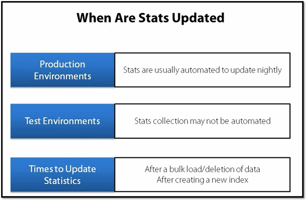
Typically, in production environments, your DBA will set up a recurring job that will keep database stats up to date, so the situation occurs less frequently. If you are in a test environment though, things may be less automated. So you want to be conscious of how current your database statistics are. Stats can also be out of date if you’ve just done a bulk load or bulk deletion of data. Since these operations can significantly change the amount of data and the distribution of data in a table. And, sometimes, after you create a new index, Oracles doesn’t seem to have very good information about that index. So it may not use that index in all the situations it should. Technically, from Oracles 10g onward, you’re not supposed to have to regather stats after creating a new index. But I’ve personally seen some situations where I’ve got some strange results. So I’ve gotten into the practice of gathering stats after creating a new index. Just to be on the safe side.
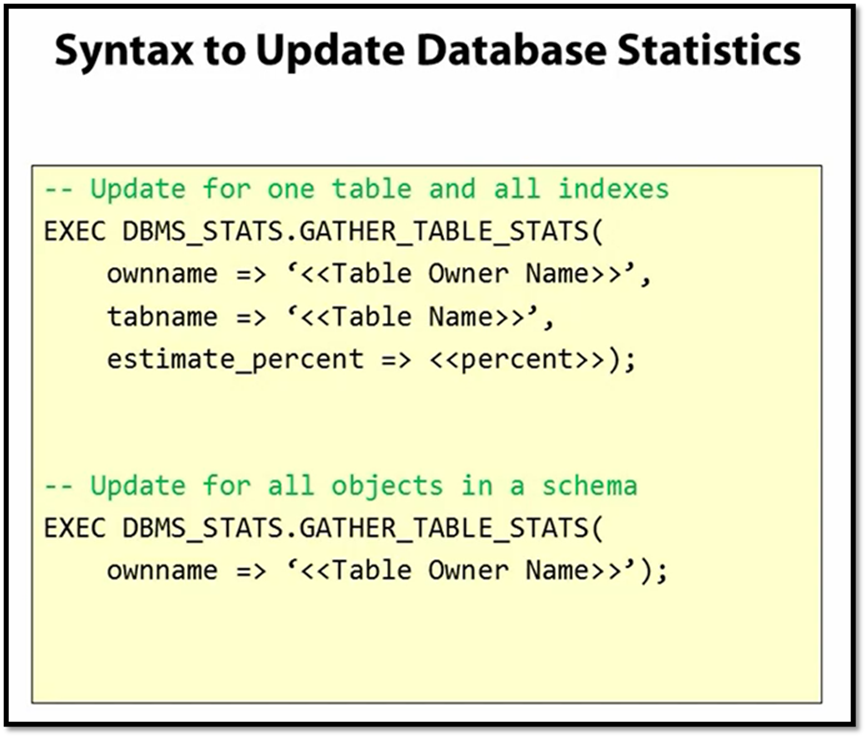
If you are concerned about your stats being out of date, the solution to get up to date stats is very simple. You just want to use the DBMS stats package. You gather your stats on a table as shown in the top item and this will cascade down to all indexes on the table as well. If the table is particularly large and you just want to sample a percentage of the rows, this can be done as well to speed up the gathering stats process. If you want to gather stats on every object in a schema, you can do that with the syntax at the bottom of the slide. You prepare, though, that if we have a large schema with a lot of tables, this could take considerable time. Whatever route you choose though, having up-to-date statistics will allow the Oracle Optimizer to make the most informed decisions about how it should execute your SQL statement. And many times, out-of-date stats are the reason why Oracle will seemingly refuse to use an index.
One of the most important practices in writing applications that use an Oracle database is to always use bind variables in your SQL statements. While easy to do, far too often this practice is not understood, or overlooked. The advantage of using bind variables is that if a query is executed multiple times, Oracle does not need to expend resources to create an execution plan each time but instead can reuse the original execution plan. This saves a lot of resources, especially CPU resources on the database server because most applications execute a relatively small number of statements over and over again. Just as important, when Oracle is able to reuse an execution plan you avoid creating contention around some segments of shared memory in the Oracle database. If this contention does occur, it creates a bottleneck around how fast SQL statements can be processed throughout the entire database. Which not just increases the amount of time it takes to process each statement, but also can greatly diminish the overall throughput of your Oracle database. Finally, using bind variables also provides protection against SQL injection attacks. And while this is a security benefit rather than a performance benefit, it is still an important consideration. Especially because SQL injection attacks always seem to be near the top of the list of application security threats.
SQL STATEMENTS AND EXECUTION PLANS
If we examine of the life of a SQL statement, we are reminded that for every SQL statement Oracle executes, Oracle must have an execution plan which tells Oracle all the individual steps that must be performed in order to process the query. This execution plan is created by the Oracle Optimizer and is shown in below step two of this diagram.
When the Oracle Optimizer creates an execution plan for a SQL statement, it must examine all of the different ways that it can process that statement in order to come up with the most efficient one. The first part of this process is for Oracle to gather all of the information about the tables involved and any indexes that could potentially be used from the Oracle Data Dictionary. To read this data, internally the Oracle Optimizer will execute over 50 queries against data dictionary objects and possibly more depending upon the complexity of the SQL statement it is attempting to analyze. Then the Optimizer takes all this data and evaluates all of the ways in which the SQL statement could be performed. This part of the process includes evaluating database statistics in order to make decisions about if an index should be used, how to perform any join operations, to what order the table should be joined in. The final phase is to take the most efficient plan and store it in an area of shared memory known as the shared SQL area. In real time this process happens very quickly. However, parsing SQL and determining the best execution plan does tend to be CPU intensive. And you also have to remember, Oracle isn’t just processing a single SQL statement at a time. It is processing hundreds or perhaps thousands of statements every second. Taken together, parsing all of these SQL statements can take up a significant amount of system resources, especially CPU.
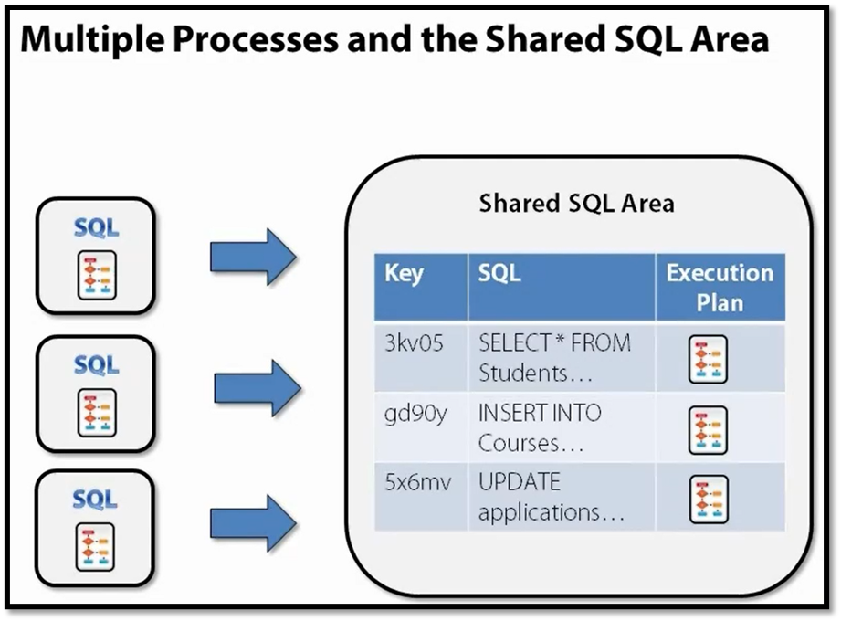
SHARED SQL AREA
The shared SQL area is a segment of shared memory in the database where Oracle caches execution plans. You can think of the shared SQL area as being similar to a large hash table. For each SQL statement, Oracle will calculate a unique key by using a hashing function and then store the parsed SQL and the execution plan in the shared SQL area by that key. The amount of memory allocated to the shared SQL area is finite. So Oracle manages the shared SQL area using a least recently used algorithm. This means that execution plans that haven’t been executed recently will be removed from the cache in order to make room for new incoming plans. Therefore, at any given time, the contents of the shared SQL area will vary. Frequently execute statements will most likely always be present. In SQL statements that are only executed a few times a day tend to have a shorter life span and be removed from the cache.
When a SQL statement is submitted to Oracle and the Oracle Optimizer needs to determine an execution plan, we will first examine the shared SQL area to see if an execution plan already exists for this SQL statement. To do this, Oracle will use the same hashing function, to calculate the hash key on the text of the submitted SQL statement. And then, much like you would in a hash table, performing a lookup by this hash key in the shared SQL area. If a matching execution plan is found, Oracle can simply read this execution plan out of the shared SQL area and continue on processing the query. If a matching execution plan is not found, then the Oracle Optimizer will go ahead and generate an execution plan for the SQL statement.
Why is Oracle cache execution planned in this way? The short answer is that generally applications contain a relatively small number of unique SQL statements and they just execute these same SQL statements over and over again with different parameters each time. By caching SQL statements and their execution plans, we see two benefits. First, we save computing resources on the database server, because we don’t have to regenerate an execution plan each time. And this frees up these resources to perform other work in our database, like actually processing our SQL statements. Second, we’ll actually see each SQL statement run slightly faster after its first execution. The reason for this is because looking up an execution plan in the shared SQL area is faster than regenerating a plan from scratch. Oracle’s not the only database to make use of caching SQL statements and their execution plans in this way. While some of the implementation details vary, you will find the same strategy used in all the major relational database systems in use today.
When Oracle is able to match an incoming SQL statement to an execution plan that is already in the shared SQL area, this is called a soft parse in Oracle terminology. If Oracle has to generate a new execution plan for a SQL statement, this is called a hard parse. You will see the terms soft parse and hard parse used consistently throughout the Oracle documentation, books written about Oracle, and blog posts. So it is important to be familiar with these terms. There will always be some level of hard parsing that needs to go on for an Oracle database. After all, there will always be a first time when a statement is submitted to Oracle, and on that first time Oracle will have to hard parse the statement. The idea though, is to minimize the amount of hard parses you do and maximize the amount of soft parsing that goes on. You should check how much hard parsing your system is doing and what the ratio is between hard parsing and soft parsing. Being able to monitor the ratio on a system-wide level gives you a good idea of the health of your Oracle database and lets you understand if there are any bottlenecks forming due to a high hard parse count. It is hard parsing that we want to avoid and make sure that Oracle can soft parse as many of our statements as possible.
There are a few loose ends about the shared SQL area that we need to spend a moment to wrap up. First, you might be wondering about the size of the shared SQL area and how many statements can be cached? The answer is that the size will vary from system to system, based on parameters, like how much memory is available in Oracle, some configuration parameters set by the DBA. But generally speaking, the shared SQL area is sized sufficiently that it can contain several thousand SQL statements and their execution plans. Second, it is important to know that the shared SQL area is shared across all users and all applications that are using a single Oracle instance. So if you have multiple applications that are using a single Oracle database as a back-end, all those applications are using the same shared SQL area. This has implications. Because if one application is doing a lot of hard parsing, it can by itself create a lot of contention around the shared SQL area and this will, in turn, affect other applications that are using that same Oracle database. Third, if you regenerate statistics on a database object, whether a table or an index, Oracle is smart enough to invalidate any execution plans that use that object, and remove those execution plans from the shared SQL area. The reason why, is that now that new statistics are available, the Oracle Optimizer may determine a different execution plan is more efficient. So we don’t want to keep that old execution plan around. This is something that Oracle manages for you internally and no action is required on your part. Finally, there’s a way for a DBA to manually flush the shared SQL area while Oracle is running and remove all of the cached SQL statements and their execution plans. Something that you probably never want to do on your production server. But it can be useful in test environments if you’re running some sort of performance test and you want to make sure that you’re starting from the same point each time.
CONTENTION AND LATCH WAITS
There’s a second impact to having a large amount of hard parsing going on in your Oracle database. This impact is more subtle, but just as serious to consider. Oracle is a multi-user system, and at any given time there are many different SQL statements being processed by Oracle. If multiple processes are all hard parsing SQL statements, then each of these processes needs access to update the shared SQL area. And here in lies the problem. So if you have multiple processes, they’re all accessing and modifying a shared data structure at the same time. That data structure will become corrupt, and the shared SQL area is no exception. Therefore, in order to protect data integrity, Oracle needs to synchronize access to the shared SQL area amongst all these different processes.
If you’ve ever done any multi-threaded programming, you’re already familiar with this concept. And object that needs to accessed and modified by multiple threads has to be protected, such that only one thread is accessed in the object at a time. In C sharp this is done using the lock keyword and in Java we use the synchronize keyword. As a result, the compiler creates a critical section of code and a serialization construct is created to make sure that only one thread can be running in that section of code at a time. In this way, the object is prevented from becoming corrupted because only one thread can be in the critical section of code modifying the object at any time. In addition, while the thread is accessing a critical code section, no other thread can read data from the object. Just make sure that no other threads read the object while it is being modified and potentially receive incomplete or inconsistent data. All of these same concepts apply in Oracle. In Oracle, we use the term latch to describe the serialization construct used to synchronize access to a shared resource. The process that currently has access to the shared resource has the latch. A process that is waiting to gain access to the shared resource is said to be undergoing a latch wait. There are a number of resources that need to be shared across processes in Oracle and therefore there are many different latches. For now though, we’ll concentrate on the latch used to synchronize access to the shared SQL area. Understanding multi-threaded operations, how locking works and why it is needed is a very difficult subject area to understand and understanding the shared SQL area is no exception to this rule. Therefore, we’ll start out with an analogy to help us understand what’s happening here.
This analogy is very similar to what happens in Oracle when multiple processes are trying to hard parse SQL statements at the same time. Just like in our file example, we can’t have all these processes writing to the shared SQL area at the same time. So this is where Oracle introduces a latch, to make sure that only one of these processes is modifying the shared SQL area, at any given time. All the other processes that need to access to shared SQL area, will experience a latch wait. In this way, Oracle is able to protect the shared SQL area from becoming corrupted, like our file did in the file example. The trade off is though, that waiting on a latch to become available, is in and of itself a very expensive operation.
When an Oracle process tries to acquire a latch but is unable to, the process that is waiting for the latch does not go to sleep and then check again after some period of time, or go into a queue where it simply waits. Instead, the waiting process undergoes what is termed Latch Spinning, where it stays on the CPU and continually checks over and over again if it can acquire the latch. The reason why Oracle does this is because going to sleep and giving up the CPU, and then getting back onto the CPU has a high cost. So if at all possible, the process wants to continue to loop and see if it can acquire the latch. So what is happening here is even though that the process is waiting, it is consuming CPU while its looping. And this is CPU that isn’t really doing any useful work. At some point, usually after 2, 000 iterations, the waiting process will give up trying to get the latch and put itself to sleep for a short period of time. When a process gives up the CPU like this and is replaced by another process, this activity is known as a context switch in operating system terminology. If you’ve studied operating systems, you know that context switching is something that you want to avoid, this is a lot of computational cost in switching from one process to another on the CPU. After a brief period of time, the process will wake up and will again be switched back into running status. At this point, it will try to acquire the latch again. And if the latch is unavailable, say a different process has acquired the latch while our waiting process was sleeping, then the Latch Spinning starts all over again. The waiting process will loop, consume CPU while trying to acquire the latch, and then potentially go to sleep again. And this cycle will continue until the process is able to acquire the latch.
What should be clear from this discussion is that contention is something that we want to do everything we can to avoid. First, because of how processes will spin while undergoing latch waits, we’re going to end up using a lot of CPU while these processes loop on the CPU. And this is CPU resources that are just wasted, not available to do other useful work in our database. The second impact of contention, is that we’re really introducing a bottleneck into our system. Statements will only process as fast as they can gain access to the shared SQL area. And as we have discussed, if we have a lot of hard parsing going on, now the responsiveness of these statements is impacted, because they have to spend time waiting to get access to the shared SQL area. One of the side effects of this bottleneck, is that we understand that a system will only run as fast as its slowest component. So it doesn’t matter how many CPUs we have, how much memory we add, or how fast our SAN is. It is this bottleneck that is going to limit the performance and the throughput of our system. What we have here is the computer science equivalent to sending all of our SQL statements down a one lane road. It doesn’t matter that we have a 12 lane super highway on the other side. Our ultimate throughput is limited by this single lane road, that is gaining access to the shared SQL area, and all of our SQL statements need to travel down this road. So clearly, if we can design applications that avoid contention in the database, we want to learn how to do this.
MATCHING SQL STATEMENTS
In the last few segments, we’ve come to understand the affects that excessive hard parsing can have on the performance of your system. Let’s now turn our attention to how to write SQL statements that will be soft parsed rather than hard parsed, and how we can incorporate these statements into our applications. For an incoming SQL statement to be matched to a SQL statement and execution plan already in the shared SQL area, the two statements have to match exactly. This includes column order, the order of predicates in your WHERE clause, and even extends to white-space characters in the statement, and what characters are in upper and lowercase. You can think of this as if you called String. Equals on the two strings of the SQL statements, one string being the incoming SQL, and the other string being the statement in the shared SQL area. If String. Equals would return true, then the statements match. In effect, what we have here is a character by character comparison of the two strings. And only if each and every character matches are the two SQL statements considered to be equivalent. Let’s take a look at a few examples of this.
On this slide, we have two queries that are each retrieving grades for a student in a particular term. And in this case, the student and the term is the same between these two queries. These two queries are exactly the same, except for the fact that in the first query, the name of the view is in all lower case. While on the second query, the name of the view is in all upper case. For the purpose of determining if the two SQL statements match, character casing counts. And so Oracle would regard these two SQL statements as different statements, and would hard parse each one.
In this slide, we have two SQL statements that are very similar to the one shown in the last slide. And once again, we’re querying the view for grades of a particular student. Notice however, that the order of columns is different between the two queries. So even though these two queries are in fact returning the same columns and therefore the same data, the fact that the column lists are in different orders means that Oracle will regard these two queries as different, and hard parse each one. It is important to consider though, that when we write an application, that we define the SQL our application uses in some sort of string in the data access class. And then we’ll use this string almost like a template that we plug values into and generate the SQL we’re going to run against the database over and over again. So generally speaking, we don’t see issues where a statement is run once in uppercase and the next time in lowercase and things like that. It’s just important to be aware of, that Oracle does match these statements exactly. And you do want to pay attention to all of the little details like character casing, column order and spacing, especially if you have any code that dynamically generates SQL.
What is more important for us to focus on, is that using literal values directly in SQL statements, causes the statements to differ, and therefore be hard parsed. Let’s see what we mean by this. Consider the two SQL statements shown on the slide. Once again, each of these statements is querying the view to get student grades for a particular semester, in this case the Fall of 2013. The only difference is that they are querying the grades for two different students. Query on the top is getting the grades for student 12345, and the query on the bottom is getting the grades for student 67890. Functionally, these two queries are exactly the same. They are returning the same columns in the same order. They have the same predicates in the WHERE clause. The only difference is which student grades will be returned for. However, since these queries are directly specifying the student ID in the WHERE clause as a literal value, Oracle will see this two queries as separate and distinct queries, and will hard parse each one. The reason why is because we have specified the literal value of the value we want in the query directly. And again, if we called String. Equals on these two strings, we would get false. So in the eyes of Oracle, these two statements will be regarded as different.
This applies not just to the student_id field, but to any literal value that can vary in any predicate in the WHERE clause. In this case, I’ve changed the query so that in both instances, we’re retrieving grade data for student 12345. The first query is getting grades for the Fall of 2013 term, and the second query, for the Spring of 2013 term. Again, these two queries are functionally equivalent, we’re just varying the term in which we are retrieving grades for. However, Oracle will again see these two SQL statements as different statements, and hard parse both of these. You can start to see the road we are headed down here. If we write our SQL statements with literal values like this, every time a different student logs on to our web application to check their grades, or a student checks their grades for a different semester. We’re going to end up with what Oracle considers a unique SQL statement, and wind up hard parsing that statement. And as we’ve talked about, that is the situation we want to avoid.
What we need to do, is to rewrite our query using Bind Variables. To do so, we’re going to replace the literal values in our WHERE clause with this syntax that represents a Bind Variable. In Oracle, the syntax that is used is a colon character followed by the name of the Bind Variable. So you can see in this statement, we’re specifying two Bind Variables, one for student_id, and one for the term_code. When Oracle parses this statement, it sees the bind variables in the text of the SQL statement, and not the actual values. So therefore, the text of the SQL statement is the same each time. Consequently, the statement will be soft parsed on each time it is run after its initial execution. What we want to do is to use a bind variable for any value in the WHERE clause that can vary on different executions of the statement. In this case, we would expect that both the student_id and the term_code would vary as the statement is run on behalf of different students looking at their grades in different terms. So both of these values need bind variables. When you submit a SQL statement that uses bind variables, you will also need to provide the actual values that Oracle will need to plug in when it executes the statement.
There are a couple of final items that we need to cover. First, pretty much all of the major object relational mappers in use today, already use bind variables implicitly. So, if you were using entity framework or in hibernate. Your application is already using bind variables and you should be in good shape. If you are using an ORM, you might be tempted to think that bind variables is a topic you don’t need to worry about. However, while new development might be taking place using an ORM, a lot of times we have to support existing applications in our jobs. And you want to make sure that these applications that are just using plain old ADO. net or JDBC are using bind variables as well. And if they’re not, you want to get those applications uplifted. One reason why that we just covered is the security concerns around SQL injection attacks. The other reason is that if you have one or two of these applications out there in your organization these applications by themselves can use up a lot of resources on your Oracle server. And cause contention around the shared SQL area. So, in that way, these existing applications that don’t use good practices can impact the performance of all of your other applications that are using that same Oracle instance.
CREATE ROLE perf_viewer;

GRANT SELECT ON V_$LOCK TO perf_viewer;
GRANT SELECT ON V_$LOCKED_OBJECT TO perf_viewer;
GRANT SELECT ON USER_OBJECT_USAGE TO perf_viewer;
GRANT SELECT ON V_$SESSION TO perf_viewer;
GRANT SELECT ON V_$SESSION_LONGOPS TO perf_viewer;
GRANT SELECT ON V_$SESSMETRIC TO perf_viewer;
GRANT SELECT ON V_$SESSTAT TO perf_viewer;
GRANT SELECT ON V_$SQL TO perf_viewer;
GRANT SELECT ON V_$SQLAREA TO perf_viewer;
GRANT SELECT ON V_$SQLSTATS TO perf_viewer;
GRANT SELECT ON V_$SQLTEXT TO perf_viewer;
GRANT SELECT ON V_$SQLTEXT_WITH_NEWLINES TO perf_viewer;
GRANT SELECT ON V_$SQL_PLAN TO perf_viewer;
GRANT SELECT ON V_$SQL_PLAN_STATISTICS TO perf_viewer;
GRANT SELECT ON V_$SQL_PLAN_STATISTICS_ALL TO perf_viewer;
GRANT SELECT ON V_$SQL_WORKAREA TO perf_viewer;
GRANT SELECT ON V_$STATNAME TO perf_viewer;
GRANT SELECT ON V_$SYSSTAT TO perf_viewer;
GRANT SELECT ON V_$TRANSACTION TO perf_viewer;

GRANT perf_viewer TO <<user name>>;